Optimization Algorithm Visualization

First let’s start with gradient descent. Well, I will not be going into the basics of optimization algorithms. I hope you are familiar with these terms already.

Parameters,

Gradient Descent

Well, I am going into the details of gradient descent. I will directly write the formula. Basically, we are trying to minimize the loss moving opposite to the direction of gradient. You are free to use resources to learn about gradient descent if you are not familiar.

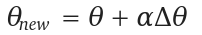where, alpha is the learning rate.

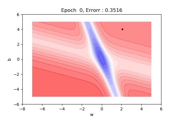
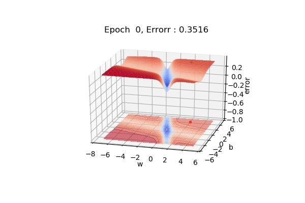
2d View

Here, the figure below shows the contour maps on 3d surface. Basically, we have plotted the weight (w), bias(b) against the error. And simply we want to find the values of w and b such that, the error is minimized. This can be any loss function. The visualization shows the red regions have high error surfaces whereas the blue regions show low error surfaces.

As we see the number of epochs increases we move downhill to the blue surface where error is low. That is what gradient descent performs. Well, if you are thinking there is a straight path but it seems that gradient descent is using other longer paths, that’s because that is the principled way to move in the direction of gradients.

That was on a 3d surface. If you see the same thing on a 2d surface, it might be a bit easy to visualize. Here you can see we are moving towards the blue contour region where the loss is minimum.

That was gradient descent. Feel free to use the resources at the end of this article to learn more how it actually works and why it works.

Momentum Based Gradient Descent

One of the observations we can take out from gradient descent is it takes a lot of time to navigate the flat regions where there is gentle slope. Suppose, we set 500 as max iterations, if the region is flat it might not be able to come out of that region and we will be stuck in local minima.

One intuitive solution for that slow move is,If I am repeatedly being asked to move in the same direction, then I should gain more confidence and start taking bigger steps : Just as the ball rolling down a slope.

Well, to write this particularly in equation it looks like :

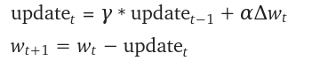
This basically means that 3 guys are already moving in that direction, so let’s take bigger steps in the same direction, maybe that direction makes sense. Lets accumulate the gradients and move in that direction.

3d Visualization

Here, you can see because of the momentum we are moving fast in the gentle slope areas too. It is much much faster than gradient descent.

There might be a caveat that, we might jump across the global minimum. One intuitive example is, suppose you are moving to a cinema hall and someone points to the direction you are moving, you move in that direction, again u ask someone he says the same direction you moving, well because of momentum you will accelerate and might pass the destination because of the high momentum, then you need to take U-turn comeback and start again.

This might be a possible scenario in case of Momentum based gradient descent.

The visualization below exactly shows the same problem that we discussed.

1. Momentum based gradient descent oscillates in and out of the minima as momentum carries it out.
2. Takes a lot of U-turns before finally convergence.
3. Despite these U-turns, it is fast than gradient descent.

Nesterov Accelerated Gradient Descent.

The idea of Nesterov Based gradient descent is, LOOK BEFORE YOU LEAP

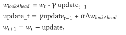
This is the update rule for momentum based gradient descent.

Here, a two steps movement is happening. First we move according to the history and second according to the current gradient.

So far in Momentum based gradient descent, we are going to move by at least and the bit more by

Can we visualize what improvement could be done here ?

Well, the idea is to calculate the gradients after moving ,

i.e what we are saying is, first lets partially update the value and then calculate the gradients as compared to momentum based, we were moving two steps and calculating gradients.

The equation for Nesterov accelerated gradient descent would look like :

Now, let’s look at the visualization. This clearly shows that we are not taking as much U-turns as we used to take in Momentum based gradient descent. This is because we are not moving two steps as in Momentum based, first we move partially, calculate gradient and then move into that direction.

In this blogpost we will limit ourself with these 3 algorithms. In the next article, we will focus on RMSProp, Adam and AdaGrad.

Resources

This blog post is heavily inspired by the lectures of Mithesh khapra from IIT Madras. Please find the lecture videos below.

1. nptel Deep Learning Lectures
2. Accompanying notebook